Calculate Correlation Between Two Stocks
Explore how we can easily see how correlated two stocks are.

A useful tool to identify help our investment decisions is the ability to assess how correlated two stocks are. Correlation is used primarily in statistics to measure how linearly related two variables are. In essence this measures how two stocks move in relation to one another.
A popular use of this idea is to perform “Pair Trading”. I have developed this tutorial to be used for long term investments.The idea is that comparing a stock e.g. AAPL to SPY (An ETF that tracks the S&P500) can be used in tandem with Forecasting, Technical Analysis or Fundamental Analysis to make a well informed investment.
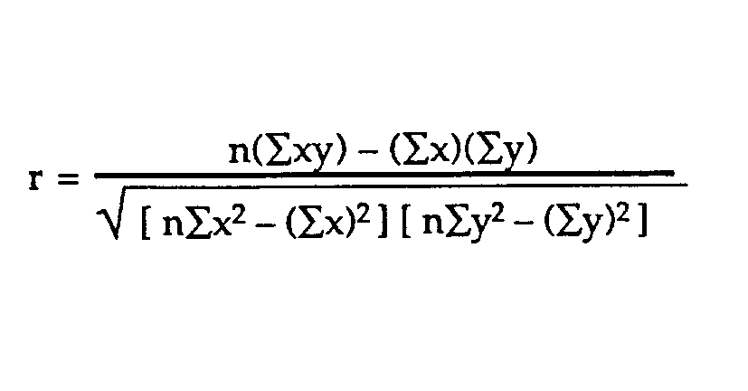
The Correlation coefficient can be calculated using the formula:

Luckily we do not have to use this formula instead a handy python library called pandas will calculate this for us.The resulting co-efficient will range from -1 to 1, -1 being perfectly negatively correlated i.e. if Stock A rises then Stock B goes down and 1 being perfectly positively correlated i.e. Stock A falls Stock B also falls.Perfect correlations are very rarely seen.
CODE
To begin we will import our dependencies, this is a simple project so we dont need that many
import yfinance as yf
import pandas as pd
import statistics
import numpy as np
yfinance is an incredibly powerful library utilizing Yahoo Finance, that makes it incredibly easy to scrape stock data including prices, fundamentals etc.
spy = yf.Ticker("SPY")
spy_hist = spy.history(period="1y")
For the purpose of this project I will be deducing how correlated AAPL is to SPY. Here we are scraping SPY’s historically data from the last year. Nothing too difficult so far.

The function in yfinance .history() will return the Open,High,Low,Close,Volume,Dividends and Stock Splits information as we see here.
aapl = yf.Ticker("AAPL")
aapl_hist = aapl.history(period="1y")
We then repeat the same step to ascertain Apples stock prices from the past year.
spy_dataframe = pd.DataFrame.from_dict(spy_hist)
aapl_dataframe = pd.DataFrame.from_dict(aapl_hist)
Following this, we want to convert our dictionaries to pandas dataframes as they will be easier to calculate the correlation later on.
spy_dataframe = spy_dataframe.pct_change()
aapl_dataframe = aapl_dataframe.pct_change()
All values are converted in both dataframes to percent changes using the .pct_change() function. We do this as these values are easier to work with when it comes to correlations, as it gives us a clearer idea of how much the stock moved relative to its price.
spy_dataframe.drop(['Volume','Dividends','Stock Splits'], axis=1)
aapl_dataframe.drop(['Volume','Dividends','Stock Splits'], axis=1)
We do not have any use for these columns so at this point we can drop them.
correlation = spy_dataframe['Close'].corr(aapl_dataframe['Close'])
print("Correlation is: ", correlation)correlation2 = spy_dataframe['Open'].corr(aapl_dataframe['Open'])
print("Correlation is: ", correlation2)correlation3 = spy_dataframe['High'].corr(aapl_dataframe['High'])
print("Correlation is: ", correlation3)correlation4 = spy_dataframe['Low'].corr(aapl_dataframe['Low'])
print("Correlation is: ", correlation4)
Here we calculate the correlation of the Close,Open, High and Low stock prices separately. Returned is 4 different correlation values which we will then combine into a Numpy array and calculate the mean giving us the total correlation coefficient.
total = np.array([[correlation],[correlation2],[correlation3],[correlation4]])
np.mean(total)
Result: 0.7536462602233308
Meaning AAPL has a very high positive correlation to SPY. This makes sense as SPY consists of 6.68% AAPL stock, the highest weight of any stock in SPY.
Conclusion
There we have it!
You have just calculated the correlation of two stocks.
This is a very general tutorial and really only meant for beginners, this should help you in understanding some basic Python and data science practices tied to stocks.
Hope you enjoyed, Happy Investing.
